On the Biases in the Estimation of Inequality Using Bracketed

On the Biases in the Estimation of Inequality Using
Bracketed Quantile Contributions
Nassim Nicholas Taleb⇤ , Raphael Douady†
⇤ Retired
† Risk
option trader, NYU Engineering
Data, Centre d’Economie de la Sorbonne
I. I NTRODUCTION
as

bq ⌘
Pn
i=1
Xi >ĥ(q) Xi
Pn
i=1
Xi
where ĥ(q) is the estimated exceedance
Pn threshold for the
probability q, i.e., ĥ(q) = inf{h : n1 i=1 x>h  q}. We
shall see that the observed variable 
bq is a downward biased
estimator of the true ratio q , the one that would hold out of
sample, and such bias is in proportion to the fatness of tails
and, for very fat tailed distributions, remains significant, even
for very large samples.
FT
Abstract—In fat-tailed domains, sample measures of top centile
contributions to wealth are biased, unstable estimators extremely
sensitive to sample size and concave in taking into account large
deviations. They tend to vary over time merely from the increase
of sample space, thus providing the illusion of structural changes
in inequality. They are also inconsistent under aggregation. In
addition, it can be shown that under fat tails, increases in
wealth need to be accompanied with increased measurement of
inequality. We compute the bias and standard error and show
some small sample and asymptotic properties of the estimator
and propose alternative extrapolative measurements of inequality
and fat-tailedness.
Let X be a random variable belonging to the class of
distributions with a "power law" right tail, that is:
P(X > x) ⇠ L(x) x
D
RA
Vilfredo Pareto noticed that 80% of the land in Italy
belonged to 20% of the population, and vice-versa, thus both
giving birth to the power law class of distributions and the
popular saying 80/20. The self-similarity at the core of the
property of power laws [1] and [2] allows us to recurse and
reapply the 80/20 to the remaining 20%, and so forth until one
obtains the result that the top percent of the population will
own about 53% of the total wealth.
It looks like such measure of inequality can be seriously
biased, depending on how it is measured, so it is very likely
that the true ratio of inequality, that is, the share of the
top percentile was closer to 70%, hences changes year-onyear would drift higher to converge to such level from larger
sample. In fact, as we will show in this discussion, more
complete samples resulting from technological progress, and
also from population and economic growth will make such a
measure converge by increasing over time, for no other reason
than expansion in sample size.
The core of the problem is that, for the class one-tailed
fat-tailed random variables, that is, bounded on the left and
unbounded on the right, where the random variable X 2
[xmin , 1), the in-sample quantile contribution (to income or
wealth) is a biased estimator of the true value of the actual
quantile contribution. Let us define the quantile contribution
II. E STIMATION
E[X|X > h(q)]
q = q
E[X]
where h(q) = inf{h 2 [xmin , +1) , P(X > h)  q} is the
exceedance threshold for the probability q.
For a given sample (Xk )1kn , its "natural" estimator 
bq ⌘
q th percentile
,
used
in
most
academic
studies,
can
be
expressed,
total
↵
(1)
where L : [xmin , +1) ! (0, +1) is a slowly varying
function, defined as limx!+1 L(kx)
L(x) = 1 for any k > 0. We
assume independent observations.
There is little difference for small exceedance quantiles
(<50%) between the various possible distributions such as
Dagum,[3],[4] Singh-Maddala distribution [5], or straight
Pareto.
For exponents 1  ↵  2, as observed in [6], the
law of large numbers operates, though extremely slowly. The
problem is acute for ↵ around (but above) 1 and severe as no
convergence is possible at 1.
A. True value of estimator
Let us first consider ↵ (x) the density of a ↵-Pareto
distribution bounded from below by xmin > 0, in other words:
xmin ↵
↵
↵ 1
.
↵ (x) = ↵xmin x
x xmin , and P(X > x) =
x
Under these assumptions, the cutpoint of exceedance is h(q) =
xmin q 1/↵ and we have:
R1
✓
◆
x (x)dx
↵ 1
h(q) 1 ↵
h(q)
q = R 1
=
=q ↵
x
x
(x)dx
min
x
min
If the distribution of X is ↵-Pareto only beyond a cut-point
xcut , which we assume to be below h(q), so that we have
P(X > x) = x ↵ for some
> 0, then we still have
h(q) = q 1/↵ and
q =
↵
↵
1 E [X]
q
↵ 1
↵
The estimation of q hence requires that of the exponent ↵ as
well as that of the scaling parameter , or at least its ratio to
the expectation of X.
In the general case, let us fix the threshold h and define:
q,h = q
E[X|X > h]
E[X]
kHSXi +YL
0.626
0.624
so that we have q = q,h(q) . We also define the n-sample
estimator:
Pn
X
Pn Xi >h i

bq,h ⌘ i=1
i=1 Xi
0.622
where Xi are n independent copies of X.
20
B. Unusal Concavity-Driven Bias of the Estimator
40
60
80
100
Y
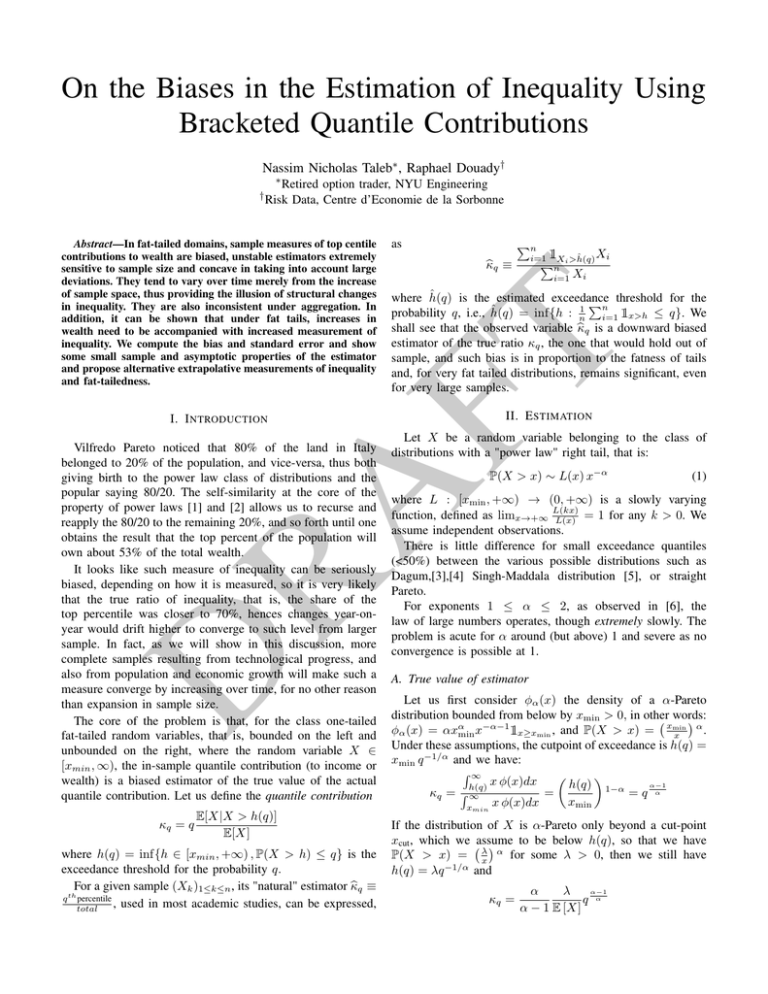
Remark 1. Let X = (X)ni=1 a random sample of size n > 1q ,
YP an extra single random observation, and define: XtY
=
q,h
Figure 2. Effect of additional observations on , we can see convexity on
both sides of h except for values of no effect to the left of h, an area of order
1/n
@ 2 XtY
q,h
 0.
@Y 2
Note that, this inequality is still valid with q as the value
hXtY (q) doesn’t depend on the particular value of Y >
hX (q).
first estimating the distribution parameters (↵, ) and only
then, estimating the tail contribution q . Falk observes that,
even with a proper estimator, the convergence is extremely
slow, of the order of n /ln n, where the exponent depends
on ↵ and on the tolerance of the actual distribution vs. a
theoretical Pareto, measured by the Hellinger distance. In
particular, ! 0 as ↵ ! 1, making the convergence really
slow for low values of ↵. The next section shows how much
the bias still remains for very large samples.
has:
Xi >h Xi + Y >h Y
P
n
i=1 Xi +Y
. We observe that, whenever Y > h, one
FT
n
i=1
RA
Unlike the common small sample effect resulting from high
impact from the rare observation in the tails less likely to show
up in small samples, a bias which goes away by repetition of
sample runs, we face a different situation. The concavity of
the estimator constitutes a upper bound for the measurement
in finite n, clipping large deviations, which leads to problems
of aggregation as we will state below in Theorem 1. This
kHSXi +YL
0.95
0.90
0.85
D
0.80
0.75
0.70
0.65
20 000
40 000
60 000
80 000
Y
100 000
Figure 1. Effect of additional observations on 
remark is probably one of the reasons why, as observed in
[7], 
bq is a non-converging estimator of q : only the number
of exceedences of a well chosen sequence of thresholds is able
to produce a converging estimator of the two key parameters
to estimate q , namely the exponent ↵ and the scale .
In practice, even in very large sample, the contribution of
very large rare events to q prevents the sample estimator to
converge to the true value. One needs to use a different path,
C. Bias and Convergence
The table below shows the bias of 
bq as an estimator of
q in the case of an ↵-Pareto distribution with ↵ = 1.1,
a value chosen to be compatible with practical economic
measures, such as the wealth distribution in the world or in
a particular country, including developped ones.1 In such a
case, the estimator is extemely sensitive to "small" samples,
"small" meaning in practice 108 . We ran a trillion simulations
across varieties of sample sizes. While .01 ⇡ 0.657933, even
a sample size of 100 million remains severely biased as seen
in Table I.
Naturally the bias is rapidly (and nonlinearly) reduced for ↵
further away from 1, and becomes weak in the neighborhood
of 2. It is also weaker outside the top 1% centile, hence this
discussion focuses on the famed "one percent" and on the low
↵ exponent.
III. A N I NEQUALITY A BOUT AGGREGATING I NEQUALITY
For the estimation of the mean of a fat-tailed r.v. (X)ji , in
m sub-samples of size n0 each for a total of n = mn0 , the
allocation of the total number of observations n between i
and j does not matter so long as the total n is unchanged.
Here the allocation of n samples between m sub-samples
does matter because of the concavity of .2 Next we prove
1 This value, which is lower than the estimated exponents one can find in
the literature – around 2 [?] – is, still according to [?], a lower estimate which
cannot be excluded from the observations.
2 The same concavity – and general bias – applies when the distribution is
lognormal.
Table I
B IASES OF E STIMATOR OF  = 0.657933 F ROM 1012 M ONTE C ARLO
R EALIZATIONS

b(n)

b(103 )

b(104 )

b(105 )

b(106 )

b(107 )

b(108 )
Mean
Median
0.405235
0.485916
0.539028
0.581384
0.591506
0.626525
0.367698
0.458449
0.516415
0.555997
0.575262
0.606915
STD
across MC runs
0.160244
0.117917
0.0931362
0.0853593
0.0601528
TK
IV. M ORE W EALTH I MPLIES I NCREASE IN ̂
INCOMPLETE SECTION (Where we show that since
the distribution is fat tailed, the maximum is of the same
order as the sum, hence additional wealth means more
measured inequality. It is quite absurd to assume that
wealth is coming from the bottom or even the middle.)
k Hn=104 L
1.0
FT
that global inequality as measured by 
bq on a broad set of
data will appear higher than local inequality, so aggregating
European data, for instance, would give a 
bq higher than the
average measure of inequality across countries – an "inequality
about inequality". In other words, we claim that the estimation
bias when using 
bq (n) is even increased when dividing the
sample into sub-samples and taking the weighted average of
the measured values 
bq (ni ).
Finally, it is easy to show that, with fat-tailed distributions, we
have E [Si /S] ni /n, again due to the fact that, conditionnaly
to a given total sum S, large sample values in a sub-sample
Ni have a higher impact on the ratio Ri than small values,
inducing a convexity effect leading to this inequality.
Putting these three inequalities together yields the result.
E [b
q (N )]
m
X
ni
i=1
Proof. Denote by S =
X
j2Ni
0.8
0.7
0.6
0.5
0.4
0.3
RA
Theorem 1. Partition the n data into m sub-samples
Pm N =
N1 [. . .[Nm of respective sizes n1 , . . . , nm , with i=1 ni =
n, and assume that the distribution of variables Xj is the same
in all the sub-samples. Then we have:
0.9
n
X
n
E [b
q (Ni )]
Xj and, for each sub-sample, Si =
j=1
Xj , so that we have S =
m
X
Si . Also denote h = hN (q)
i=1
D
for the full sample and, for each sub-sample, hi = hNi (q).
Then we have:
m
X
Si

bq,h (N ) =

bq,h (Ni )
S
i=1
We first observe that, in each sample:
E [b
q,h (Ni )]
60 000
E [b
q,hi (Ni )]
This is simply due to the fact that the larger the ratio 
bq,h (Ni ),
the higher hi is likely to be, hence reducing the contribution
of the "tail" of Ni beyond hi to the total sum Si .
The second observation is that, for a given threshold h, the
random variables Ri and 
bq,h (Ni ) are positively correlated,
indeed, conditionally to a given upward bias of Ri with respect
to its expectation, due to fat tails, the bias is more likely
due to a large contribution of the tail beyond h than to an
accumulation of values above average but below h. Hence we
have:


Si
Si

bq,h (Ni )
E
E [b
q,h (Ni )]
E
S
S
80 000
100 000
120 000
Wealth
Figure 3. Effect of additional wealth on ̂
V. C ONCLUSION AND P ROPER E STIMATION OF
I NEQUALITY
Inequality can be severe at the level of the generator, but in
small n we observe a lower . So we get a historical illusion
of rise in wealth inequality when it has been there all along.3
Even the estimation of ↵ can be biased in some domains
where one does not see the entire picture: in the presence
of uncertainty about the "true" ↵, it can be shown that, unlike
other parameters, the one to use is not the probability-weighted
exponents (the standard average) but the minimum across a
section of exponents [6].
It did not escape our attention that some theories are
built based on claims of such "increase" in inequality, as
in [9], without taking into account the true nature of ,
and promulgating theories about the "variation" of inequality
without reference to the stochasticity of the estimation and
the lack of consistency of . We also faced the argument that
"the sudy is based on a complete set of data" and estimating
in sample ̂ from "robust" methods works. Robust methods,
alas, tend to fail with fat-tailed data.
Take an insurance (or, better, reinsurance) company. The
"accounting" profits in a year in which there were few claims
do not reflect on the "economic" status of the company. The
3 Accumulated
wealth is typically thicker tailed than income,[8].
"accounting" profits are not used to predict variations year-onyear, rather the exposure to tail (and other) events, analyses
that take into account the stochastic nature of the performance. This difference between "accounting" (deterministic)
and "economic" (stochastic) values matters for policy making,
particularly under fat tails.
How Should We Measure Inequality?
ACKNOWLEDGMENT
FT
Risk managers now tend to compute CVaR and other
metrics, methods that are extrapolative and nonconcave, such
as the information from the ↵ exponent (taking the one from
the lower bound of the range of exponents) and rederiving
the corresponding , are less biased and do not get mixed up
with problems of aggregation.4 By extrapolative, we mean the
built-in extension of the tail in the measurement by taking into
account realizations outside the sample path that are in excess
of the extrema observed.5
The late Benoît Mandelbrot, Dominique Guéguan, Felix
Salmon, Bruno Dupire, the staff at Luciano Restaurant in
Brooklyn and Naya in Manhattan.
R EFERENCES
D
RA
[1] B. Mandelbrot, “The pareto-levy law and the distribution of income,”
International Economic Review, vol. 1, no. 2, pp. 79–106, 1960.
[2] ——, “The stable paretian income distribution when the apparent
exponent is near two,” International Economic Review, vol. 4, no. 1,
pp. 111–115, 1963.
[3] C. Dagum, “Inequality measures between income distributions with
applications,” Econometrica, vol. 48, no. 7, pp. 1791–1803, 1980.
[4] ——, Income distribution models. Wiley Online Library, 1983.
[5] S. Singh and G. Maddala, “A function for size distribution of incomes:
reply,” Econometrica, vol. 46, no. 2, 1978.
[6] N. N. Taleb, “Silent risk: Lectures on fat tails,(anti) fragility, and
asymmetric exposures,” Available at SSRN 2392310, 2014.
[7] M. Falk et al., “On testing the extreme value index via the pot-method,”
The Annals of Statistics, vol. 23, no. 6, pp. 2013–2035, 1995.
[8] X. Gabaix, “Power laws in economics and finance,” National Bureau of
Economic Research, Tech. Rep., 2008.
[9] T. Piketty, “Capital in the 21st century,” 2014.
[10] T. Piketty and E. Saez, “The evolution of top incomes: a historical and
international perspective,” National Bureau of Economic Research, Tech.
Rep., 2006.
4 Some authors such as [10] use Pareto interpolation for unsufficient
information about the tails (based on tail parameter), filling-in the bracket
with conditional average bracket contribution, which is not the same thing as
using full power-law extension, hence retains the bias.
5 Even using a lognormal distribution, by fitting the scale parameter, works
to some extent as a rise of the standard deviation extrapolates probability mass
into the right tail.
THIS IS FROM N N TALEB’S “SILENT RISK” AS APPENDIX SHOWING
PROBLEMS IN ESTIMATION OF TAIL ALPHAS UNDER PARAMETER
UNCERTAINTY
4
Effects of Higher Orders of
Uncertainty
Chapter Summary 4: The Spectrum Between Uncertainty and Risk.
There has been a bit of discussions about the distinction between "uncertainty" and "risk". We believe in gradation of uncertainty at the level
of the probability distribution itself (a "meta" or higher order of uncertainty.) One end of the spectrum, "Knightian risk", is not available for
us mortals in the real world. We show how the effect on fat tails and
on the calibration of tail exponents and reveal inconsistencies in models
such as Markowitz or those used for intertemporal discounting (as many
violations of "rationality" aren’t violations .
4.1
Meta-Probability Distribution
When one assumes knowledge of a probability distribution, but has uncertainty attending the parameters, or when one has no knowledge of which probability distribution to
consider, the situation is called "uncertainty in the Knightian sense" by decision theorisrs(Knight, 1923). "Risk" is when the probabilities are computable without an error
rate. Such an animal does not exist in the real world. The entire distinction is a lunacy,
since no parameter should be rationally computed witout an error rate. We find it preferable to talk about degrees of uncertainty about risk/uncertainty, using metadistribution,
or metaprobability.
The Effect of Estimation Error, General Case
The idea of model error from missed uncertainty attending the parameters (another layer
of randomness) is as follows.
Most estimations in social science, economics (and elsewhere) take, as input, an average
or expected parameter,
Z
↵=
↵ (↵) d↵,
(4.1)
where ↵ is distributed (deemed to be so a priori or from past samples), and regardless of
the dispersion of ↵, build a probability
distribution for x that relies on the mean estimated
⇣
⌘
parameter, p(X = x)= p x ↵ , rather than the more appropriate metaprobability
adjusted probability for the density:
Z
p(x) =
(↵) d↵
(4.2)
91
92
CHAPTER 4. EFFECTS OF HIGHER ORDERS OF UNCERTAINTY
Prob
0.1
%ni!1 p #X Αi $ Φ i
p#X Α# $
0.001
10$5
"
10
p!X Α"
$7
X
5
50
10
500
100
1000
Figure 4.1: Log-log plot illustration of the asymptotic tail exponent with two states.
In other words, if one is not certain about a parameter ↵, there is an inescapable layer
of stochasticity; such stochasticity raises the expected (metaprobability-adjusted) probability if it is < 12 and lowers it otherwise. The uncertainty is fundamentally epistemic,
includes incertitude, in the sense of lack of certainty about the parameter.
The model bias becomes an equivalent of the Jensen gap (the difference between the
two sides of Jensen’s inequality), typically positive since probability is convex away from
the center of the distribution. We get the bias !A from the differences in the steps in
integration
✓ Z
◆
Z
!A =
(↵) p(x|↵) d↵ p x| ↵ (↵) d↵
With f (x) a function , f (x) = x for the mean, etc., we get the higher order bias !A0
! A0 =
Z ✓Z
(↵) f (x) p(x|↵) d↵
◆
dx
Z
✓ Z
◆
f (x) p x| ↵ (↵) d↵ dx
(4.3)
Now assume the distribution of ↵ as P
discrete n states, with ↵ = (↵i )ni=1 each with
n
associated probability = i _i=1^n,
i=1 i = 1. Then 4.2 becomes
p(x) =
i
n
X
i=1
p (x |↵i )
!
(4.4)
So far this holds for ↵ any parameter of any distribution.
4.2
Metadistribution and the Calibration of Power Laws
Remark 1. In the presence of a layer of metadistributions (from uncertainty about
the parameters), the asymptotic tail exponent for a powerlaw corresponds to the lowest
possible tail exponent regardless of its probability.
4.2. METADISTRIBUTION AND THE CALIBRATION OF POWER LAWS
93
This explains "Black Swan" effects, i.e., why measurements tend to chronically underestimate tail contributions, rather than merely deliver imprecise but unbiased estimates.
When the perturbation affects the standard deviation of a Gaussian or similar nonpowerlaw tailed distribution, the end product is the weighted average of the probabilities.
However, a powerlaw distribution with errors about the possible tail exponent will bear
the asymptotic properties of the lowest exponent, not the average exponent.
Now assume p(X=x) a standard Pareto Distribution with ↵ the tail exponent being
estimated, p(x|↵) = ↵x ↵ 1 x↵
min , where xmin is the lower bound for x,
p(x) =
n
X
↵i x
↵i 1 ↵i
xmin i
n
X
↵i x
↵i 1 ↵i
xmin i
i=1
Taking it to the limit
limit x↵
⇤
+1
x!1
=K
i=1
where K is a strictly positive constant and ↵⇤ = min ↵i . In other words
1in
↵⇤ +1
Pn
i=1
↵i x
↵i 1 ↵i
xmin i
is asymptotically equivalent to a constant times x
. The lowest parameter in the space
of all possibilities becomes the dominant parameter for the tail exponent.
P"x
0.0004
0.0003
0.0002
Bias ΩA
0.0001
STD
1.3
1.4
1.5
1.6
1.7
1.8
Figure 4.2: Illustration of the convexity bias for a Gaussian from raising small probabilities:
The plot shows the STD effect on P>x, and compares P>6 with a STD of 1.5 compared to P>
6 assuming a linear combination of 1.2 and 1.8 (here a(1)=1/5).
Pn
Figure 4.1 shows the different situations: a) p(x|↵), b) i=1 p (x |↵i ) i and c) p (x |↵⇤ ).
We can see how the last two converge. The asymptotic Jensen Gap !A becomes p(x|↵⇤ )
p(x|↵).
Implications
Whenever we estimate the tail exponent from samples, we are likely to underestimate
the thickness of the tails, an observation made about Monte Carlo generated ↵-stable
variates and the estimated results (the “Weron effect”)[74].
The higher the estimation variance, the lower the true exponent.
94
CHAPTER 4. EFFECTS OF HIGHER ORDERS OF UNCERTAINTY
The asymptotic exponent is the lowest possible one. It does not even require estimation.
Metaprobabilistically, if one isn’t sure about the probability distribution, and there is
a probability that the variable is unbounded and “could be” powerlaw distributed, then
it is powerlaw distributed, and of the lowest exponent.
The obvious conclusion is to in the presence of powerlaw tails, focus on changing
payoffs to clip tail exposures to limit !A0 and “robustify” tail exposures, making the
computation problem go away.
4.3
The Effect of Metaprobability on Fat Tails
Recall that the tail fattening methods in 2.4 and 2.6.These are based on randomizing
the variance. Small probabilities rise precisely because they are convex to perturbations
of the parameters (the scale) of the probability distribution.
4.4
Fukushima, Or How Errors Compound
“Risk management failed on several levels at Fukushima Daiichi. Both TEPCO and its
captured regulator bear responsibility. First, highly tailored geophysical models predicted an infinitesimal chance of the region suffering an earthquake as powerful as the
Tohoku quake. This model uses historical seismic data to estimate the local frequency
of earthquakes of various magnitudes; none of the quakes in the data was bigger than
magnitude 8.0. Second, the plant’s risk analysis did not consider the type of cascading,
systemic failures that precipitated the meltdown. TEPCO never conceived of a situation
in which the reactors shut down in response to an earthquake, and a tsunami topped the
seawall, and the cooling pools inside the reactor buildings were overstuffed with spent
fuel rods, and the main control room became too radioactive for workers to survive, and
damage to local infrastructure delayed reinforcement, and hydrogen explosions breached
the reactors’ outer containment structures. Instead, TEPCO and its regulators addressed
each of these risks independently and judged the plant safe to operate as is.”Nick Werle,
n+1, published by the n+1 Foundation, Brooklyn NY
4.5
The Markowitz inconsistency
Assume that someone tells you that the probability of an event is exactly zero. You ask
him where he got this from. "Baal told me" is the answer. In such case, the person is
coherent, but would be deemed unrealistic by non-Baalists. But if on the other hand,
the person tells you "I estimated it to be zero," we have a problem. The person is
both unrealistic and inconsistent. Something estimated needs to have an estimation
error. So probability cannot be zero if it is estimated, its lower bound is linked to the
estimation error; the higher the estimation error, the higher the probability, up to a
point. As with Laplace’s argument of total ignorance, an infinite estimation error pushes
the probability toward 12 . We will return to the implication of the mistake; take for now
that anything estimating a parameter and then putting it into an equation is different
from estimating the equation across parameters. And Markowitz was inconsistent by
starting his "seminal" paper with "Assume you know E and V " (that is, the expectation
and the variance). At the end of the paper he accepts that they need to be estimated, and
what is worse, with a combination of statistical techniques and the "judgment of practical
men." Well, if these parameters need to be estimated, with an error, then the derivations