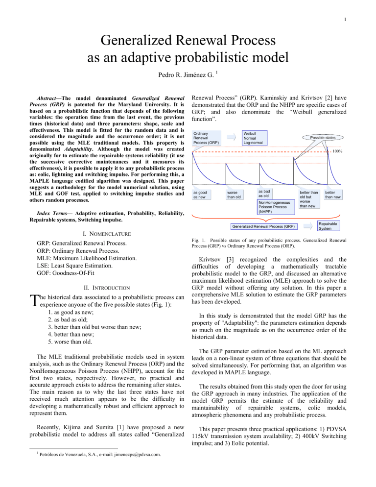
1 Generalized Renewal Process as an adaptive probabilistic model Pedro R. Jiménez G. 1 Abstract—The model denominated Generalized Renewal Process (GRP) is patented for the Maryland University. It is based on a probabilistic function that depends of the following variables: the operation time from the last event, the previous times (historical data) and three parameters: shape, scale and effectiveness. This model is fitted for the random data and is considered the magnitude and the occurrence order; it is not possible using the MLE traditional models. This property is denominated Adaptability. Although the model was created originally for to estimate the repairable systems reliability (it use the successive corrective maintenances and it measures its effectiveness), it is possible to apply it to any probabilistic process as: eolic, lightning and switching impulse. For performing this, a MAPLE language codified algorithm was designed. This paper suggests a methodology for the model numerical solution, using MLE and GOF test, applied to switching impulse studies and others random processes. Index Terms— Adaptive estimation, Probability, Reliability, Repairable systems, Switching impulse. Renewal Process” (GRP). Kaminskiy and Krivtsov [2] have demonstrated that the ORP and the NHPP are specific cases of GRP; and also denominate the “Weibull generalized function”. Ordinary Renewal Process (ORP) Weibull Normal Log-normal 100% as good as new worse than old as bad as old NonHomogeneous Poisson Process (NHPP) Generalized Renewal Process (GRP) I. NOMENCLATURE GRP: Generalized Renewal Process. ORP: Ordinary Renewal Process. MLE: Maximum Likelihood Estimation. LSE: Least Square Estimation. GOF: Goodness-Of-Fit T II. INTRODUCTION he historical data associated to a probabilistic process can experience anyone of the five possible states (Fig. 1): 1. as good as new; 2. as bad as old; 3. better than old but worse than new; 4. better than new; 5. worse than old. The MLE traditional probabilistic models used in system analysis, such as the Ordinary Renewal Process (ORP) and the NonHomogeneous Poisson Process (NHPP), account for the first two states, respectively. However, no practical and accurate approach exists to address the remaining after states. The main reason as to why the last three states have not received much attention appears to be the difficulty in developing a mathematically robust and efficient approach to represent them. Recently, Kijima and Sumita [1] have proposed a new probabilistic model to address all states called “Generalized 1 Petróleos de Venezuela, S.A., e-mail: jimenezps@pdvsa.com. Possible states better than old but worse than new better than new Repairable System Fig. 1. Possible states of any probabilistic process. Generalized Renewal Process (GRP) vs Ordinary Renewal Process (ORP). Krivtsov [3] recognized the complexities and the difficulties of developing a mathematically tractable probabilistic model to the GRP, and discussed an alternative maximum likelihood estimation (MLE) approach to solve the GRP model without offering any solution. In this paper a comprehensive MLE solution to estimate the GRP parameters has been developed. In this study is demonstrated that the model GRP has the property of "Adaptability": the parameters estimation depends so much on the magnitude as on the occurrence order of the historical data. The GRP parameter estimation based on the ML approach leads on a non-linear system of three equations that should be solved simultaneously. For performing that, an algorithm was developed in MAPLE language. The results obtained from this study open the door for using the GRP approach in many industries. The application of the model GRP permits the estimate of the reliability and maintainability of repairable systems, eolic models, atmospheric phenomena and any probabilistic process. This paper presents three practical applications: 1) PDVSA 115kV transmission system availability; 2) 400kV Switching impulse; and 3) Eolic potential. 2 III. THE MODEL A. Description (6) The Cumulative Density Function (CDF) or unreliability function of the GRP model is as in (1): β ⎡ i −1 ⎞ ⎤ ⎛ ⎢ tj ⎟ ⎥ β ⎜ t i +q ⎢ ⎛ q i −1 ⎞ ⎜ ⎟ ⎥ j=1 ⎢⎜ ⎟ ⎥ t j ⎟ −⎜ η ⎢ ⎜ η j=1 ⎟ ⎜ ⎟ ⎥ ⎠ ⎜ ⎢⎝ ⎟⎟ ⎥ ⎜ ⎢ ⎠ ⎥⎦ ⎝ ⎣ ∑ F(t i , β, q, η) = 1 − e ∑ ,t≥0 (7) (1) The parameters are: η = scale , β = shape and q = effectiveness. The “β” parameter have the cases: β < 1 (early life), β = 1 (userful life) and β > 1 (wearout life). The “q” parameter have the cases: q = 0 (as good as new), q = 1 (as bad as old), 0 < q < 1 (better than old but worse than new), q < 0 (better than new) and q > 1 (worse than old). (8) The Probability Density Function (PDF) is as in (2): (9) β ⎡ i −1 ⎛ ⎞ ⎤ ⎢ tj ⎟ ⎥ β ⎜ t +q ⎢ ⎛ q i −1 ⎞ ⎜ i ⎟ ⎥ j 1 = ⎢⎜ ⎟ ⎥ t j ⎟ −⎜ ⎢ ⎜ η j=1 ⎟ ⎜ η ⎟ ⎥ ⎠ ⎜ β−1 ⎢ ⎝ ⎟⎟ ⎥ ⎜ ⎢ ⎝ ⎠ ⎥⎦ ⎣ ∑ ∑ i −1 ∂F(t i ) ⎛ β ⎞⎛ ⎞ = ⎜⎜ β ⎟⎟⎜ t i + q ∑ t j ⎟ e f(t i , β, q, η) = (2) j=1 ⎠ ∂t i ⎝ η ⎠⎝ The hazard function (failure rate fuction) is as in (3): β −1 i −1 ⎛ β ⎞⎛ f (t i ) ⎞ λ(t i , β, q, η) = = ⎜ ⎟⎜ t i + q ∑ t j ⎟ (3) j=1 1 − F( t 1 ) ⎜⎝ ηβ ⎟⎠⎝ ⎠ B. Algorithm The MLE Weibull model F( t ) = 1 − e solving the equations system as in (4) ∂ ln(L) ∂ ln(L) (β, q) = 0, (β, q) = 0, η = η(β, q) (11) ∂β ∂q β is obtained 1 ⎛ n β ⎞β x βi ln(x i ) ∑ ln(x i ) ⎜ ∑ xi ⎟ ∑ 1 i =1 i =1 ⎜ i =1 ⎟ (4) 0 , − − = η = n ⎜ n ⎟ n β β xi ⎜ ⎟ ∑ i =1 ⎝ ⎠ n n The GRP MLE model is obtained solving the equations system as in (7), (8) and (9) equaling to zero. Applying MLE: n L = f(t1 , β, q, η)∏ f(t i , β, q, η) (10) Substituting (10) en (7) y (8), is obtained a nonlinear equation system, dependent of β y q, as in (11). The algorithm is divided in three phases: a) Weibull MLE model. b) GRP MLE model. c) LSE Weibull model is fitted to MLE GRP model. ⎛t⎞ − ⎜⎜ ⎟⎟ ⎝ η⎠ From (9), equal to zero, is solved as in (10): (5) i=2 Applying natural logarithm (Ln) and expanding, it is obtained (6). The numeric calculus of (11) imply the solution from two planes, due the asymptotic form for β = 1, as: Solution #1. Plane 0 < β < 1 y - ∞ < q < ∞. Recommended Initial Conditions: q = 0.0001 y β = 0.5. b) Solution #2. Plane 1 < β < ∞ y - ∞ < q < ∞. Recommended Initial Conditions: q = 0.2 y β = 3. Note: the recommended initial conditions are the result of rehearsals, although in general it is subjected to verification. a) To know the best solution is necessary apply the Kolmogorov-Smirnov (KS) test (or any other GOF test): ( KS = maximum F( t i ) − ni , F( t i ) − ( i −1) n ), i = 1..n The smallest KS test value is the best solution. In case that the MLE GRP model doesn't have solution, the Weibull MLE model is assumed as solution. 3 For simplify calculus and interpretation, is accepted to fit the MLE GRP model to the Weibull model F(t) = 1 − e applying LSE, according to the following steps: 1. 2. 3. β The dependent values are the times and the independent values are the GRP function evaluated for each time. With the data of the step 1, the LSE is applied for solving the parameters β and η. To be initialized it assumes a value of the parameter γ. The step 2 is repeated, varying the parameter γ, until to maximize the R2 statistical test: ⎛ n ⎞ R = 1 − ⎜ ∑ ( y i − ŷ i ) 2 ⎟ ⎝ i =1 ⎠ 2 4. ⎛ t −γ ⎞ −⎜⎜ ⎟⎟ ⎝ η ⎠ n ⎛ n ⎞ ⎜ ∑ y i − ∑ y j n ⎟ (12) ⎜ ⎟ i 1 j 1 = = ⎝ ⎠ Conservative criterions. If the data have reliability philosophy (is less probable long times) then the parameter γ should be ≤ 0 (if LSE is γ > 0, should be recalculated for γ=0). For maintainability philosophy (is more probable long times) the parameter γ should be ≥ 0. The MLE traditional models are: For compare the MLE traditional models with the MLE GRP model, is apply any GOF test as Kolmogorov - Smirnov (KS). This test value should be smallest that the critical values for 1% statistical significance. The GRP model prospective time “P”, is obtained as in (18) and (19). Be (18) the CDF for the next time (tn+1). ∑ F(t n +1 ) = 1 − e ∞ δ −∞ −δ P = ∫ f(t)dt = ∫ ⎛t⎞ ∂ F(t n +1 ) dt n +1 ∂ t n +1 (19) ∫ δ −δ t 2n +1 ∂ F(t n +1 ) dt n +1 − µ 2 ∂ t n +1 (20) (13) Generally, it is expressed in percentage of the prospective time. Note: δ substitute at infinite for numeric calculation. Range: 50η to 1000η. (14) The algorithm developed is codified in the MAPLE language. The nonlinear equations system is resolved using the “Newton” library. Normal: 1 ⎛ t −µ ⎞ ⎟ σ ⎠ (18) The deviation “D” is as in (20). β − ⎜ 1 f (t) = e 2⎝ 2π ⋅ σ ,t ≥ 0 Applied to reliability study is called mean life or “Mean Time To failure” (MTTF) and applied to maintainability is called “Service Outage Mean Time” (SOMT). D= ∂F( t ) ⎛ β ⎞ β−1 −⎜⎜⎝ η ⎟⎟⎠ ,t ≥ 0 = ⎜⎜ β ⎟⎟(t ) e ∂t ⎝η ⎠ ∑ Then, the prospective time “P” (or average time) is as in (19). Weibull: f (t) = β ⎡ n ⎞ ⎤ ⎛ ⎢ +q t j ⎟ ⎥ β ⎜t ⎢ ⎛ q n ⎞ ⎜ n +1 ⎥ ⎟ j=1 ⎢⎜ ⎟ ⎥ t j ⎟ −⎜ η ⎢ ⎜ η j=1 ⎟ ⎜ ⎥ ⎟ ⎠ ⎜ ⎢⎝ ⎟⎟ ⎥ ⎜ ⎢ ⎠ ⎥⎦ ⎝ ⎣ 2 ,−∞ < t < ∞ C. Why is said that the GRP model is adaptive? Be the data according to the occurrence order: LogNormal: f (t) = 1 ⎛ ln t −µ ⎞ ⎟ σ ⎠ − ⎜ 1 e 2⎝ 2π ⋅ t ⋅ σ 2 ,t ≥ 0 (15) and the ascending order data: Then, the results are shown in the table I. TABLE I ADAPTABILITY PROPERTY Extreme Value (EV): ⎛ t −µ ⎞ ⎟ σ ⎠ 1 −⎜ f (t) = e ⎝ σ 2 e e 2 ⎛ t −µ ⎞ −⎜ ⎟ ⎝ σ ⎠ −∞ < t < ∞ (16) This Extreme Value model is obtained solving the MLE equations system: (17) η β q P D occurrence order 794 0.697 7.91 9231 100% Ascending order 95.7 0.48 3.26 13996 102% Conclusion: the GRP model parameters estimation depends on the magnitude and the occurrence order of the data. This property is denominated Adaptability. 4 D. Availability study of the PDVSA 115kV electrical system. Hours This part is a repairable system application whose objective is to estimate the reliability (probability that a system doesn't fail for a specific time, only associated to non-programmed events) and maintainability (service restoration probability for a specific time, associated to non-programmed and programmed events) of the PDVSA 115kV electric system, with the purpose of to estimate the system availability (probability that a system is in service, associated to nonprogrammed or programmed events, whose value represents the mean for a long time) and to compare with the international standard. Maintainability (SOT) 16 14 12 10 8 6 4 2 0 1 2 3 4 5 6 7 8 9 10 11 12 13 14 15 16 17 18 19 20 21 22 23 24 25 26 27 28 29 30 31 32 33 34 35 36 37 38 39 40 41 42 43 44 45 occurrence order Fig. 3. SOT historical Data. Source: PDVSA statistics. Conclusion: The 115kV system reliability and maintainability study report the mean values of MTTF = 4477hours and SOMT = 5.12hours, respectively. The PDVSA 115kV electrical system availability (A) is calculated as in (21). MTTF 4477 100 = 100 = 99.885% (21) MTTF + SOMT 4477 + 5.12 Important: the MLE traditional models are not applicable for repairable systems availability studies. A= The data to estimate the reliability model are the times to failure (TTF), which is defined as the lapsed operative time, since a failure is restored until it is failure again. E. 400kV Switching impulse study. The data to estimate the maintainability model are the service outage times (SOT), which is defined as the lapsed time since a failure until it is restored. Hours Reliability (TTF) 30000 25000 20000 15000 GRP parameters η = 2533 hours β = 0.6368 q = 0.002218 P = 4477 hours D = 143% GRP parameters q = 0.000311 β = 1.51 η = 5.75 hours P = 5.12 hours D = 68% This part is a switching impulse application for 400kV CIGMA-Furrial transmission line with length=310Km using pre-insertion resistor and surge arrester at each terminal. This study permit to obtain the line optimal CFO (Critical Flash Over) to satisfy the Switching Forced Outage Rate (SSFOR). This study consists in the energization at the CIGMA terminal. For the study, the basic equations are as in (22) to (25): 10000 5000 0 a 1 2 3 4 5 6 7 8 9 10 11 12 13 14 15 16 17 18 19 20 21 22 23 24 25 26 27 28 29 30 31 32 33 34 35 36 37 38 39 40 41 42 43 44 45 46 47 48 49 50 51 52 53 54 55 56 occurrence order E2 = a Fig. 2. TTF historical Data. Source: PDVSA statistics. is the undervoltage value more probable. σ σf ⎞ , ⎛ CFOn = CFO⎜1 + z f ⎟ 0.03 < f < 0.07, typical = 0.05 CFO CFO ⎠ ⎝ is the equivalent CFO for n-tower. (23) TABLE II GRP MODEL SOLUTIONS COMPARISON Solution #1 2533hours 0.6368 0.002218 0.1488 Solution #2 836hours 0.6308 0.195705 0.3018 z f = inverse Normal = N −1 (1 − n _ tower 0.5 ), n_tower = Comment: the GRP model solution that best fit is the 1 , due KS1 < KS2. Simplifying to LSE Weibull: E +D 2 1 SSFOR = f ( t )dt ≤ 1 / 1000 2 CFOn=CFO∫(1+0.05zf ) (25) Note: the MAPLE program has codified these equations. TABLE III RELIABILITY LSE WEIBULL MODEL β 0.811 line length 0.4 (24) The CFO estimation is obtained numerically solving (25): st η 3797 hours (22) 0 Using the MAPLE codefied program: η β q KS test ∫ f (t )dt = 0.98, t ≥ 0 γ 0 Comment: young system, due that β = 0.811 < 1 Objective #1: to determine the CFOmin and CFOmax of each function to satisfy the SSFOR criterion < 1/1000. The MAPLE program include the estimation of: CFOmin: is obtained when the 1st function, whose KS test < critical value, reach SSFOR < 1/1000. CFOmax: is obtained when all functions, whose KS test < critical value, reach SSFOR < 1/1000. 5 TABLE VI SWITCHING IMPULSE STUDY SUMMARY Objective #2: to compare the MAPLE results between the MLE traditional models and the GRP model. GRP Random Data: The following random data (n = 149) are the phase-neutral peak under-voltage per-unit values and they are obtained through simulations applying a PSCAD switching impulse model measured at 75%line. Weibull Normal LogNormal EV E2 1.695 1.702 1.772 1.80588 P 1.489 1.496 1.492 1.492 1.503 D 0.1252 0.1258 0.1363 0.1424 0.1871 0.07386 0.0739 0.07694 0.07885 0.09409 1.82 1.828 1.908 1.948 2.175 0.1216 0.09736 D / E2 E2 + D KS test KS < CV Yes 0.1303 Yes Yes 1.988 0.1482 0.1728 No No Note: the KS critical value (CV) is 0.1335 for n = 149 and 1% statistical significance. TABLE VII CFOMIN ESTIMATION Fig. 4. MAPLE program input data (random values). Note: the MAPLE language codified algorithm filter the repeated data. GRP CFOmin TABLE IV GRP MODEL SOLUTIONS COMPARISON η β q Solution #1 1.557166 14.64 0.0000633 Solution #2 Not Exist 2.0752 775 775 775 775 775 1.751 1.751 1.751 1.751 1.751 0.001358 0.013676 0.019799 0.046042 In the table VII is show the CFOmin estimation. Comment: it demonstrate that the GRP model permit obtain the optimum CFO value. It apply for the majority of the cases. TABLE VIII CFOMAX ESTIMATION Model Extreme Value Normal LogNormal Weibull µ 1.419 1.492 0.395 - σ 0.146 0.136 0.095 - η 1.550 GRP CFOmax MLE TRADITIONAL MODELS Weibull 2.2152 n tower β 14.56 EV 2.0752 0.000939 Comment: only exist one solution for the GRP model. TABLE V LogNormal 2.0752 CFOn SSFOR Normal 2.0752 n tower To next be showing the MAPLE codified program reports. Weibull 2.0752 CFOn Normal 2.2152 LogNormal 2.2152 EV 2.2152 2.2152 775 775 775 775 775 1.869 1.869 1.869 1.869 1.869 0 0 0.000835 0.002833 0.019557 SSFOR In the table VIII is show the CFOmax estimation. It is a conservative value for design (107%CFOmin ). F. Eolic potential study of the Venezuela Oriental region. GRP parameters η = 7.89 m/s β = 6.56 q = 0.0046 P = 6.20 m/s D = 21% Eolic measurement. Venezuela Oriental Region m/s 12 10 8 6 4 2 0 1 2 3 4 5 6 7 8 9 10 11 12 13 14 15 16 17 18 19 20 21 22 23 24 25 26 27 28 29 30 31 32 33 34 35 36 37 occurrence order Fig. 6. Eolic measurement.Venezuela Oriental region. TABLE IX LSE WEIBULL MODEL η 7.936 m/s green: Extreme Value yellow: LogNormal red: GRP blue: Weibull gold: Normal Fig. 5. Probabilistic Density Function and histogram. From MAPLE program β 6.6 γ -1.2 Note: for this case, the β parameter not has interpretation. The GRP model is only applied for to fit the data. 6 Comment: the eolic potential of the Venezuela Oriental region is bigger than 5 m/s, therefore it is feasible the electric generation. IV. CONCLUSIONS a) b) c) d) e) f) g) h) PGR is a mathematical model that has the property of "Adaptability”: the parameters depend of the magnitude and the occurrence order of the historical data. It is not recommended to use the censored or suspended data for the PGR model, due the nonexistence of a defined occurrence order. The GRP model, applied to a probabilistic switching impulse study, permits the optimum CFO value estimation. Applying the GRP model for the PDVSA 115kV electrical system availability study is obtain 99.885% ≈ 99,9%, whose value is satisfactory according to recommended practice. The result β < 1 imply that the 115kV PDVSA electric system is in infantile mortality period. The “q” predominant value of the PDVSA 115kV system is approximately “as good as new” (q ≈ 0). For many data (usually for maintainability data) is accepted the MLE Weibull model. The PGR model opens a world of opportunities for the investigation of any probabilistic model as: maintenance, eolic, lightning and switching impulse. V. RECOMMENDATIONS a) It is invited to apply this PGR to more complex systems study as: refineries, compressors, large bombs, ovens, cryogenic and any repairable industrial process. b) The PGR model opens the doors to continue investigating its application with censored data. c) To verify with certainty the null hypothesis (that the model is adjusted to the data) for the function PGR, is necessary a complementary investigation for the development of an adapted goodness-of-fit test. VI. REFERENCES [1] [2] [3] [4] [5] Kijima M. y Sumita N. (1986). A useful generalization of renewal theory: counting process governed by non-negative Markovian increments. J Appl Prob 1986; 23:71–88. Kaminskiy M. y Krivtsov V. (1998). A Monte Carlo approach to repairable system relaibility analysis. Probabilistic safety assessment and management, New York: Springer; p. 1063–8. Krivtsov V. (2000). A Monte Carlo approach to modeling and estimation of the generalized renewal process in repairable system reliability analysis. Dissertation for The Degree of Doctor of Philosophy, University of Maryland. Xie, Yang y Gaudoin (2001). National University of Singapore, Singapore. Institut National Polytechnique de Grenoble, France. Regression Goodness-Of-Fit Test for Software Reliability Model Validation. Joglar F., Modarres M. y Yanez M. (2002). Reliability Engineering & System Safety. Generalized renewal process (GRP) for analysis of repairable systems with limited failure experience. Approved for University of Maryland at April 29, 2002. VII. BIOGRAPHIES Pedro Jiménez was born in Puerto La Cruz city, Venezuela country, on February 1, 1973. He graduated electrical engineer with honors from the UDO University on 1996 and Maintenance Management MSc on 2006. He has 11 years of experiences with Petróleos de Venezuela, S.A., working electrical planning, engineering and electrical simulations. He is professor of the UDO University since 1996. He has published in some national and international congresses related to power systems analysis.
