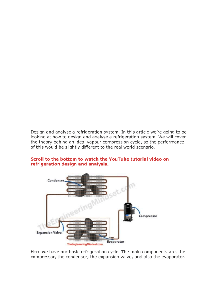
Design and analyse a refrigeration system. In this article we’re going to be looking at how to design and analyse a refrigeration system. We will cover the theory behind an ideal vapour compression cycle, so the performance of this would be slightly different to the real world scenario. Scroll to the bottom to watch the YouTube tutorial video on refrigeration design and analysis. Here we have our basic refrigeration cycle. The main components are, the compressor, the condenser, the expansion valve, and also the evaporator. The compressor compresses the refrigerant and pushes it around the system. The condenser rejects the unwanted heat from the system. The expansion valve expands the refrigerant. The evaporator absorbs the unwanted heat that’s been collected from the building, it also produces the cooling, which goes out to the building. To design and analyse a refrigeration system, we want to know what the thermodynamic properties will be for the refrigerant at our four key components. Point 1: Point 2: Point 3: valve. Point 4: between the evaporator and the compressor. as it leaves the compressor. when it leaves the condenser, before it enters into the expansion just after the expansion valve, before it enters into the evaporator. For each of these points, we need to know the refrigerants temperature, entropy, pressure, and enthalpy. We’re going to plot our system onto two charts to do this. Notice the grey line which forms a dome on both. Anything to the left of this is where the refrigerant is a liquid. Any point under the dome, the refrigerant is part vapor, part liquid mixture. Anything to the right hand side of the line is where it’s going to be a super heated vapor. If the point touches the line on the left, then it’s saturated liquid. If it touches the line on the right then it’s going to be a saturated vapor. The blue lines mark out our system performance. From the above graphs we can see that point 1 is going to be a low temperature, it’s also going to be a low pressure and it’s going to be a saturated vapor. Point 2 we can see will be a much higher pressure. It’s also a high temperature and it’s in the super heated region, so it’s a super heated vapor. Point 3 we can see is still a high pressure, it has reduced slightly in temperature, and it is also on the saturated liquid line, so it’s going to be a saturated liquid. We can also see that point 4, just after the expansion valve, when the refrigerant has been expanded, the refrigerant will be a much lower pressure and temperature. So it’s a low pressure, low temperature, and it’s in between the dome. So it’s going to be a liquid vapor mixture. We will use some acronyms: T is going to be for temperature. P is going to be for pressure. H is going to be for enthalpy. S is going to be for entropy. X will be the quality of the refrigerant. If it’s a liquid then it’s a 0, if it’s a vapor then it’s 1. We use this to work out how far between being a liquid and a vapor the refrigerant is when it’s in the dome region. M dot is the mass flow rate of refrigerant Now there’s lots of ways that you can start to design one of these systems. Probably knowing the cooling load that you want to achieve would be a very good point to start with. Refrigerant at point 1 We’re going to start with the compressor. Let’s say I have a compressor that’s able to push seven kilograms a second of refrigerant around the system. From the compressors manufacturers data, we can find that it’s able to produce a 1,200 KPA of pressure and it also needs a suction pressure of 320 KPA. So we start by using these values. We will input this data into a chart. So, we know that the suction pressure is 320 KPA and that it is a saturated vapor on the saturation line (Point 1). We just need to look up what the values of these are going to be on the thermodynamic properties of refrigerant. For this example we’ll just use R134a. You can obtain the properties for Refrigerant R-134a by clicking here Then scroll down to the saturated vapour refrigerant tables. So we want to find 320 KPA. Take a note of the values highlighted above. These at the saturated vapour conditions when the refrigerant is at 320 kPa for temperature, volume, enthalpy and entropy. These are all values for Point 1. Refrigerant at point 2 Now we’ll have a look to find what the properties of the refrigerant are at state 2. Now, go back to the refrigerant tables, we need to know two points of reference this time to find the values. At the moment we just know what the pressure is (1,200 kPa)and we know it’s a super heated vapor. Because we are doing this as an ideal cycle, we can assume the compressor is isotropic and that means the entropy at point 2 equals that at point 1. (0.9301 kJ/kg.K) We therefore input copy the entropy value from point 1 to point 2. Now we have two data points so we can look in the super heated vapor tables to find the enthalpy and temperature. Find the superheated refrigerant tables. We’re looking for 1,200 kPa. Now, the entropy we’re looking for is 0.9301 kJ/kg.K. But looking down this list, we can’t find it, it’s between two values. So to find it, we just have to use some linear interpolation. Watch the YouTube tutorial to see how to calculate this in excel. Refrigerant at point 3 As this is an ideal system, there is no resistance to flow, so there’ll be no pressure drop. In the real world obviously there will be a little pressure drop, but as this is ideal then we can assume that the pressure at point 3 is the same as point 2. Now we have the pressure and we know that it is a saturated liquid and that means we can use the saturated liquid tables to find out the temperature, enthalpy and entropy. Coming back to the property’s tables, Locate the saturated refrigerant tables and look for 1,200 kPa. We know that it’s a saturated liquid. So we want the saturated liquid columns. So copy the temperature, enthalpy and entropy values. That’s all our properties for Point 3. Refrigerant at point 4 Now we need to know what the properties of the refrigerant are going to be at point 4. This is slightly more tricky because it’s in the vapor dome. So it’s part liquid, part vapor. We’re not sure exactly yet how much vapor or liquid it is. But that’s okay because we can just work it out. We know the temperature is going to be the same as point 1 and that the enthalpy will remain constant through the expansion valve. (Look at the charts to see that). So, that means we can use the enthalpy from state 3. Therefore we can drop these figures in for point 4. We also know what the pressure is because that is going to be equal to state 1 and that means we only need to find out what the entropy is. The way we do that, is by finding the quality of the refrigerant. So what part liquid or vapor do we have. For that we come back to the saturated refrigerant tables. We scroll down until we find the 320 kPa line. Then we want to copy the entropy, enthalpy, temperature, and pressure for both the saturated liquid and vapors. Paste these into excel it’ll be easier. We find the quality using the above formula. I’ve already filled in the values. X being the quality and H representing the enthalpy. We already have the value of H4, because that was equal to the enthalpy at point 3. We also know what HF and HG are because we’ve have them here on the table. HF is the saturated liquid and HG is the saturated vapor value. When we drop the numbers into the formula, you’ll see that this comes out as a decimal, because it’s a ratio, which is roughly 32%. We now use that value to work out what the entropy is going to be at state 4, and we do that using the formula below. S4 therefore equals 0.4436 kilojoules per kilogram per Kelvin. So that’s all the properties of the refrigerant worked out. Work done by the compressor Let’s work out the amount of work done by the compressor. We can do that using this formula below. For that, we use the enthalpy of state 2 and state 1 and the mass flow rate of the refrigerant. From the formula we can see that the compressor’s doing 82.29 kilowatts of work on the system. Evaporator cooling load We can also work out the cooling load on the evaporator by using the formula below. It’s almost exactly the same formula. We’re just using the enthalpy from point 1 and the enthalpy from point 3. Using this we can see that it’s providing 402 kilowatts of cooling. Condenser heat rejection We can also calculate the heat rejection by the condenser and we can see that from the formula below. Again, a very simple and similar formula. We can see the condenser is rejectiong 485 kilowatts. Notice that is higher than the cooling provided and that’s because we have to get rid of the heat produced by the compressor as well. So you can add these together to check if your fingers are correct. If they don’t equal, then you’ve done something wrong and you need to go back and just have a look through some of your figures. Coefficient of performance We can calculate the efficiency of the system, or the coefficient of performance, using this formula below. This formula is very simply, it’s just a ratio of work out by work in. This example our system has a coefficient of performance of 4.89. Meaning for every kilowatt of electricity you put in, you’ll get 4.89 kilowatts of cooling out, which is very efficient. Here are all our properties for the system.
