Simulation of the motion of a sphere through a viscous fluid

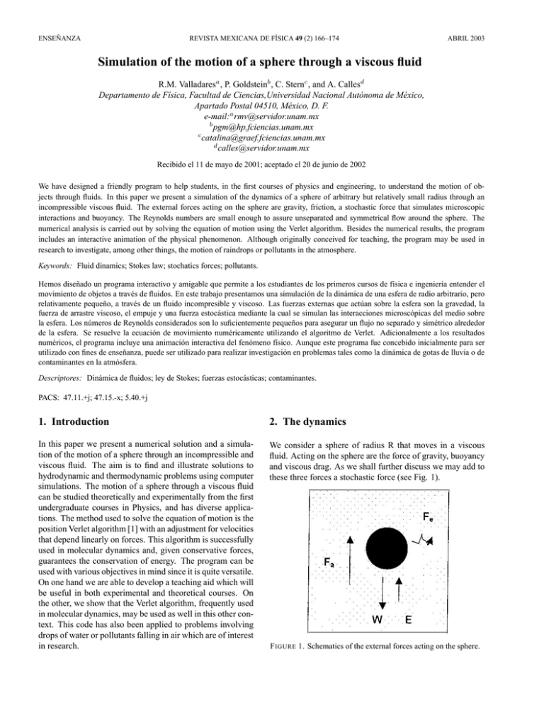
ENSEÑANZA
REVISTA MEXICANA DE FÍSICA 49 (2) 166–174
ABRIL 2003
Simulation of the motion of a sphere through a viscous fluid
R.M. Valladaresa , P. Goldsteinb , C. Sternc , and A. Callesd
Departamento de Fı́sica, Facultad de Ciencias,Universidad Nacional Autónoma de México,
Apartado Postal 04510, México, D. F.
e-mail:a rmv@servidor.unam.mx
b
pgm@hp.fciencias.unam.mx
c
catalina@graef.fciencias.unam.mx
d
calles@servidor.unam.mx
Recibido el 11 de mayo de 2001; aceptado el 20 de junio de 2002
We have designed a friendly program to help students, in the first courses of physics and engineering, to understand the motion of objects through fluids. In this paper we present a simulation of the dynamics of a sphere of arbitrary but relatively small radius through an
incompressible viscous fluid. The external forces acting on the sphere are gravity, friction, a stochastic force that simulates microscopic
interactions and buoyancy. The Reynolds numbers are small enough to assure unseparated and symmetrical flow around the sphere. The
numerical analysis is carried out by solving the equation of motion using the Verlet algorithm. Besides the numerical results, the program
includes an interactive animation of the physical phenomenon. Although originally conceived for teaching, the program may be used in
research to investigate, among other things, the motion of raindrops or pollutants in the atmosphere.
Keywords: Fluid dinamics; Stokes law; stochatics forces; pollutants.
Hemos diseñado un programa interactivo y amigable que permite a los estudiantes de los primeros cursos de fı́sica e ingenierı́a entender el
movimiento de objetos a través de fluidos. En este trabajo presentamos una simulación de la dinámica de una esfera de radio arbitrario, pero
relativamente pequeño, a través de un fluido incompresible y viscoso. Las fuerzas externas que actúan sobre la esfera son la gravedad, la
fuerza de arrastre viscoso, el empuje y una fuerza estocástica mediante la cual se simulan las interacciones microscópicas del medio sobre
la esfera. Los números de Reynolds considerados son lo suficientemente pequeños para asegurar un flujo no separado y simétrico alrededor
de la esfera. Se resuelve la ecuación de movimiento numéricamente utilizando el algoritmo de Verlet. Adicionalmente a los resultados
numéricos, el programa incluye una animación interactiva del fenómeno fı́sico. Aunque este programa fue concebido inicialmente para ser
utilizado con fines de enseñanza, puede ser utilizado para realizar investigación en problemas tales como la dinámica de gotas de lluvia o de
contaminantes en la atmósfera.
Descriptores: Dinámica de fluidos; ley de Stokes; fuerzas estocásticas; contaminantes.
PACS: 47.11.+j; 47.15.-x; 5.40.+j
1. Introduction
2. The dynamics
In this paper we present a numerical solution and a simulation of the motion of a sphere through an incompressible and
viscous fluid. The aim is to find and illustrate solutions to
hydrodynamic and thermodynamic problems using computer
simulations. The motion of a sphere through a viscous fluid
can be studied theoretically and experimentally from the first
undergraduate courses in Physics, and has diverse applications. The method used to solve the equation of motion is the
position Verlet algorithm [1] with an adjustment for velocities
that depend linearly on forces. This algorithm is successfully
used in molecular dynamics and, given conservative forces,
guarantees the conservation of energy. The program can be
used with various objectives in mind since it is quite versatile.
On one hand we are able to develop a teaching aid which will
be useful in both experimental and theoretical courses. On
the other, we show that the Verlet algorithm, frequently used
in molecular dynamics, may be used as well in this other context. This code has also been applied to problems involving
drops of water or pollutants falling in air which are of interest
in research.
We consider a sphere of radius R that moves in a viscous
fluid. Acting on the sphere are the force of gravity, buoyancy
and viscous drag. As we shall further discuss we may add to
these three forces a stochastic force (see Fig. 1).
F IGURE 1. Schematics of the external forces acting on the sphere.
167
SIMULATION OF THE MOTION OF A SPHERE THROUGH A VISCOUS FLUID
Buoyancy, given by Archimedes principle asserts that a
body in a fluid experiences an apparent reduction in weight
equal to the weight of the displaced fluid. The drag force associates all forces that resist the motion of the sphere due to
friction (viscosity) or to the motion of the fluid close to the
sphere.
In general, the drag force cannot be represented in a simple mathematical way since, besides the effect due to viscosity (viscous drag), for Reynolds numbers larger than five, the
form of the wake (form drag) is determinant in describing the
behavior of the sphere.
We recall that the Reynolds number is an adimensional
parameter that characterizes the flow and is given by
Re =
2Rvρ
,
η
(1)
where v is the uniform speed of the flow, η is the viscosity
and ρ the density of the fluid.
For small Reynolds numbers, the flow around the sphere
is symmetrical and does not separate, and the drag can be
considered to be due only to friction forces over the surface
of the sphere. Stokes [2] calculated the drag force for a static
sphere in a steady, uniform, infinite viscous and incompressible flow (or a sphere that moves through a static fluid) for
sufficiently small Reynolds numbers,
Fa = −cv = −(6πηR)v.
(2)
Parameter c is of geometric origin, and has been calculated
for geometries other than spheres.
Comparison of Eq. (2) with experiments show that for
Re< 0.5 the expression is very good and accurate to about
10% for Re close to 1 [3]. For Reynolds numbers larger than
five the wake behind the sphere gets more and more complicated as the speed increases. This form drag can be reduced
designing aerodynamic objects that diminish the wake. The
value of various geometrical factors as well as the evolution
of the wake with Reynolds numbers can be found in any introductory book of fluid mechanics [2, 4]. For solid particles
falling in air, the geometry correction is negligible. In this paper we limit our analysis to small Reynolds numbers in which
the drag is due only to viscosity, and a simple mathematical
form can be assumed.
If we consider a particle subject to gravity, buoyancy and
drag as mentioned above, the balance of the three forces will
determine whether the motion will be uniform or accelerated.
In the examples shown below, the initial motion is accelerated
and, under certain conditions, as the drag force increases with
speed the forces balance out and the particle attains terminal
(constant) speed. Equation (2) was obtained for steady conditions so in the acceleration phase additional terms must be
considered.
One of those terms is related to the resistance of the nonviscous fluid to the motion of the particle. It can be obtained
by adding a certain mass of the fluid to the true mass of the
sphere and is called virtual or added mass. Added mass effects are usually associated with bodies immersed in liquids
because their density is larger than in gases [3]. In the case
of small solid particles or raindrops falling in air the added
mass effect is of the order of 10−3 or smaller.
The other term, proposed originally by Basset, is related
to the diffusion of vorticity. It is also more important in liquids than in gases and for regimes with high Reynolds numbers. The term can be neglected in the examples that we show
below.
When the motion of fluid spheres in another fluid is considered the recirculation of the fluid at the interface might
play an important role. This is true however only for gas
bubbles in a liquid. In the case of raindrops it has been shown
that they behave like solid particles: when they are very small
Eq. (2) is valid and for higher Reynolds numbers the drag depends on the complex flow that surrounds the sphere.
In addition to the three forces mentioned above we may
propose the existence of a stochastic force that depends on
the temperature and which allows the study of cases in which
Brownian motion might be of interest. The form of this
stochastic force [5] is
·
Fe = GRAN
2ckB T
∆t
¸ 21
,
(3)
where GRAN is a random number with a Gaussian distribution centered at zero and standard deviation 1, kB is Boltzmann’s constant, T is the absolute temperature, c is the coefficient in Stokes’ formula [Eq. (2)].
In molecular dynamics it is common to use stochastic motion equations to carry out the sampling of a canonical ensemble. The dynamic equation for the sphere in one dimension is
therefore given by the following Langevin type equation [4]:
m
dv
d2 x
= m 2 = −cv + FT ,
dt
dt
(4)
where the total force FT is given by
FT = mg − V ρg + Fe ,
(5)
and c = 6πηR, V the volume displaced by the sphere and m
is the sphere’s mass.
3. The Verlet algorithm
In order to solve Eq. (4) numerically we turn to the Verlet
algorithm so frequently used in molecular dynamics [1]. We
now make a brief description of the Verlet algorithm with a
modification to account for forces that have a linear dependence on velocity such as Stokes’ drag force.
Let us call the time step of the Verlet algorithm h=∆t
where h is assumed very small compared to the normal time
scale of the problem. To calculate the position and velocity
we use a Taylor series expansion for x(t + h):
µ ¶
µ
¶
dx
1 d2 x
x(t + h) = x(t) +
h+
h2 + . . . , (6)
dt t
2 dt2 t
Rev. Mex. Fı́s. 49 (2) (2003) 166–174
168
R.M. VALLADARES, P. GOLDSTEIN, C. STERN, AND A. CALLES
and
µ
x(t − h) = x(t) −
dx
dt
¶
h+
t
1
2
µ
2
d x
dt2
to calculate x(h) we need x(-h) which we obtain from Eq. (7)
to second order:
¶
h2 − . . .
(7)
t
Adding Eqs. (6) and (7) up to second order we find
x(t + h) = 2x(t) − x(t − h) + a(t)h2 .
(8)
On the other hand subtracting Eq. (7) from Eq. (6) we find
µ ¶
dx
x(t − h) − x(t + h) = 2h
,
(9)
dt t
(10)
Since the force depends on the velocity, the position at
time t + h will depend on the velocity at time t, and this velocity requires the expression for x(t + h). If we write
where
1
b=g−
m
F (t)
= b − c0 v(t),
m
(
·
RAN
V ρg + G
¸ 21 )
2ckB T
∆t
,
and
c
m
and substitute it into Eq.(8) we have
c0 =
x(t + h) = 2x(t) − x(t − h) + [b − c0 v(t)] h2 .
(11)
Substituting eq.(10) and factorizing,
µ
¶
µ
¶
c0 h
c0 h
x(t+h) 1+
=2x(t)−x(t−h) 1+
+bh2 , (12)
2
2
we have finally that the uncoupled equations to solve by iterations are
Ã
!
c0 h
2x(t) − x(t − h) 1 +
+ bh2
2
Ã
!
x(t + h) =
(13)
1 + c0 h
2
and
x(t + h) − x(t − h)
,
(14)
2h
which constitute the modified Verlet algorithm for forces that
have a linear dependence on velocity.
For t = 0 we have
v(t) =
x(0) = 0,
v(0) = v0 ,
a(0) = a0 = g −

1
m
ρV g + c0 v0 − Gran
Ã
With these values for the initial position and velocity, iterating we can generate all the previous values for both position and velocity at time intervals of h. This algorithm, aside
from being fast and reliable, is quite compact and easy to
program [1].
4. Applications
so the expression for the velocity turns out to be:
µ ¶
dx
x(t + h) − x(t − h)
v(t) =
=
.
dt t
2h
a(t) =
1
1
x(−h)=x(0)−v(0)h+ a(0)h2 =x0 −v0 h+ a0 h2 . (15)
2
2
2ckB T
∆t
! 21 
,
In this paper two different applications of the software, that
we think are of interest to students and researchers, are considered. The results are presented in the next section. The
first phenomenon studied is the precipitation of raindrops of
different radii (from 1x10−5 to 1x10−3 m.). Each radius is
kept constant throughout the fall. However, an option for a
variable radius exists in the program, and more sophisticated
models can be easily introduced. The motion of each drop
depends on the size. The smallest drops remain floating in
the air, the middle one acquires very soon terminal speed,
and most of the trajectory has constant velocity. The bigger
drops remain in accelerated motion.
The second application refers to the motion of pollutants
in the atmosphere. Five different materials in two typical
sizes are considered. From this very simple model it can be
seen that the smallest pollutants can remain floating in the air
that we breathe for long periods of time. The stochastic force
always has a small but noticeable effect in the motion of the
pollutants.
5. Results
Using the previous equations and initial conditions, an interactive program in C language was written to calculate position and velocity as a function of time. The program was
developed for PC in MS-DOS environment, and shows an
animation of the motion. The parameters and initial conditions can be changed easily using special keys. An example of a screen that will appear to the student is shown in
Fig. 2 (see the appendix for details). The program can do up
to five numerical experiments simultaneously. Spheres are
dropped inside “tubes” filled with a particular fluid at a given
temperature. The use of the tubes is only for visual effects.
All hypotheses consider the motion of a sphere in an infinite
medium. The program has a database of ten different fluids
and twenty-four possible materials for the spheres. Table I
has the values of the densities and viscosities of the fluids in
SI units. Table II has the densities of the materials for the
spheres.
Figure 2 shows the simulation of the fall of water drops
with radii varying from 1x10−5 to 1x10−3 m. The time step
used in the integration is 0.004s. The starting point is in the
middle of the screen. The smallest drops do not seem to
Rev. Mex. Fı́s. 49 (2) (2003) 166–174
SIMULATION OF THE MOTION OF A SPHERE THROUGH A VISCOUS FLUID
169
F IGURE 2. Simulation of the fall of water drops with radii varying from 1x10-5 to 1x10-3 m.
TABLE I.
Fluid
Vacuum
Air
Water
Oil (10)
Oil (20)
Oil (30)
Oil (40)
Oil (50)
Glycerine
Helium
Density (kg/m)3
0
1.293
1000.0
910
910
910
910
910
1270
0.18
Viscosity (kg/ms)
0
0.000018
0.001
0.079
0.170
0.310
0.430
0.630
0.1
0.00001
move. They float without falling in the time scale considered.
The reason is that there is a minimum size for water drops to
precipitate. The two drops on the right are much bigger and
touch the bottom very soon: 0.464s and 0.456s as shown on
top of their respective tubes. Their Reynolds number was already high after 0.4s, and the assumption of symmetrical flow
around them was probably not valid in the last part of their
trajectory. Figures 3 and 4 show the position and speed of
the drops as a function of time. Particle 1 moves very little
with speed close to zero, particles 2 and 3 attain terminal velocity very soon, and particles 4 and 5 remain in accelerated
motion. The simulation is a close approximation only for
the first two raindrops whose motion remains at very small
Reynolds numbers. For drop number three the type of motion
is correctly described even though the actual values of the
speed and position are not accurate. The Reynolds numbers
of the last two raindrops are too big to be described by this
theory. The stochastic force due to temperature is extremely
small in these experiments, its effect can be neglected.
F IGURE 3. Position of the water drops as a function of time. For
the two smallest particles the graphs are straight lines almost from
the beginning because they soon attain terminal velocity, and move
at constant speed. The third particle starts with accelerated motion (curved line) but eventually attains terminal velocity. The two
bigger particles fall with accelerated motion all the time.
Rev. Mex. Fı́s. 49 (2) (2003) 166–174
170
R.M. VALLADARES, P. GOLDSTEIN, C. STERN, AND A. CALLES
TABLE II.
Material
Steel
Asphalt
Sulphur
Clay (1)
Clay (2)
Sand (dry)
Asbestos
Coal (M)
Coal (V)
Wax
Concrete
Cork
Glass fiber
Chalk
Graphite
Ice
Soot
Brick
Wood
Paper
Petroleum
Lead
Helium
Water
Density (kg/m)3
7850
1200
1960
1800
2600
1600
2500
1200
300
960
2400
200
100
1800
100
960
1600
1400
500
700
800
11400
0.18
1000
F IGURE 4. Velocity of the water drops as a function of time. The
speed of the first drop remains almost zero. The speed of the second is constant most of the time. The third shows a clear change of
behavior. Drops 4 and 5 move with constant acceleration
Figure 5 shows the fall in air from a height of one meter of
five different contaminants: lead, soot, sulfur, clay and coal.
All spheres have a radius of 5x10−6 m. These are typical sizes
for PM-10 pollutants in the air. The particles fall very slowly
so the integration time has been increased (0.04s). The program can be stopped either when the first or when the last
particle touches the ground. In this experiment the lead particle touched the bottom at 28.92s as can be seen at the top
F IGURE 5. Simulation of the fall in air from a height of one meter of five different PM-10 (radius of 5x10-6 m) contaminants: lead, soot,
sulfur, clay and coal.
Rev. Mex. Fı́s. 49 (2) (2003) 166–174
SIMULATION OF THE MOTION OF A SPHERE THROUGH A VISCOUS FLUID
of the corresponding tube. The other four particles are still
in the air. The instant at which they touch the ground will
appear above the positions and velocities at the top of each
tube. Their Reynolds number appears at the bottom. In the
case of variable radius, the size would be shown in this space
also. As can be seen, all Reynolds numbers correspond to
the range where our hypothesis is valid. The parameters of
the experiment appear below each tube. The total time up
to the instant when (S) was typed (31.640s) appears at the
top right corner of the screen. Figure 6 shows the graph of
speed as a function of time for each of the particles. All particles start downwards with accelerated motion. Eventually,
the drag force increases with speed, and soon the sum of the
Stokes and the buoyancy forces balances the weight. The particles seem to attain terminal speed and continue at constant
speed. However, if the proper scale is plotted like in Fig. 7, it
can be seen that there is always a small variation around the
terminal speed. This is due to the stochastic force. In Fig. 8
position is plotted as a function of time. The stochastic effect
is not observed at this scale. The graph shows straight lines
as if all particles moved at constant speed. When the particle
touches the bottom, the position remains constant.
To study the effect of the stochastic force in more detail,
the simulation might be carried out without gravity as shown
in Fig. 9. The particles oscillate about the origin, this figure
shows an instant of time. Figures 10 and 11 show the speed
and position of the particles as a function of time. The particles have a random motion about the origin with an amplitude
that seems to depend on the mass. These results are valid in
a direction perpendicular to the fall. For this simulation the
distance interval between top and bottom was reduced
171
F IGURE 7. Small variations about the terminal speed due to the
stochastic force.
F IGURE 8. Position is plotted as a function of time for PM10 particles. The stochastic effect is not observed at this scale. The graph
shows straight lines as if all particles moved at constant speed.
When the particle touches the bottom, the position remains constant.
F IGURE 6. Velocity as a function of time for each of the PM10 particles. All particles start downwards with accelerated motion. All
particles seem to attain terminal velocity, and continue at constant
speed. However, if the proper scale is plotted like in Fig. 7, it can
be seen that there is always a small variation around the terminal
speed. This is due to the stochastic force
[-5 x10−5 , -5 x10−5 m] but the same time increment (0.04s)
was used in the integration.
To study random signals it is often convenient to use statistical methods. Figure 12 shows a histogram of the position
of coal without gravity for a very long run. The histogram
shows the number of times a certain value is attained during the run. It can be observed that the highest values corresponds to the origin. The particle goes up or down randomly.
It could be expected that as we let the time go to infinity,
the peak at the origin will increase and the histogram will be
more symmetric showing that the number of times the particles goes above the origin is the same as the number of times
it goes below.
Rev. Mex. Fı́s. 49 (2) (2003) 166–174
172
R.M. VALLADARES, P. GOLDSTEIN, C. STERN, AND A. CALLES
F IGURE 9. Simulation of the motion of PM10 particles without gravity.
lead particles will remain in the air for over 12 minutes, but
the ones made out of the four other materials will take over
an hour to touch the ground. In the case of the smaller PM2.5
pollutants, the lead ones will remain in the air over 3 hours
but the other materials will remain floating between 20 to 30
hours if emitted by a tall chimney. If we consider only the
first 3m above the ground, where we breathe, the less dense
particles will remain in the air over 2 hours. Thus, these
smaller particles may be considered hazardous to health and
represent one of the main causes of air pollution.
F IGURE 10. Position of PM-10 particles without g as a function of
time. The particles have an erratic motion whose amplitude seems
to depend on the mass.
The speeds and positions for the fall of smaller contaminants, PM-2.5 (with a radius of 1.25 x 10−6 m.) are shown
in Figs. 13 and 14. These particles being smaller fall more
slowly, and the effect of the stochastic force can be detected
in the velocity. All positions start as a curve as in accelerated
motion but eventually become straight lines.
If we consider that pollutants are ejected into the atmosphere by chimneys about 25m high, using the data obtained
in the simulation we can conclude the following. The 5µ
F IGURE 11. Velocity of PM-10 particles without g as a function of
time.
Rev. Mex. Fı́s. 49 (2) (2003) 166–174
SIMULATION OF THE MOTION OF A SPHERE THROUGH A VISCOUS FLUID
F IGURE 12 A . Position of PM-2.5 (radius of 1.25 x10-6 m) particles as a function of time. The particles have an erratic motion
whose amplitude seems to depend on the mass.
173
F IGURE 14. Velocity of PM-2.5 particles as a function of time. The
particles have an erratic motion superposed to the fall. Note that the
speed diminishes before it becomes approximately constant.
It is interesting to note that even this simple model gives
information on phenomena studied by meteorologists.
6. Animation as a teaching tool
The teacher can use the software presented in this paper in
various ways.
F IGURE 12 B . Histogram corresponding to Fig. 12a. The highest
frequency corresponds to the origin.
1. In early undergraduate Physics courses, students may
easily compare experimental measurements of different falling spheres in different fluids with the numerical
predictions. At this level we recommend eliminating
the stochastic term. This program is friendly enough
to allow students to change the parameters according
to the real experiments that may be achieved in the lab.
This experience will enable students to understand the
utility of “numerical” experiments as useful tools to
plan actual experiments, determine the best parameters
to be used in the laboratory, and predict results.
2. In an advanced course, the stochastic term may be included and the student may visualize the numerical
results of a stochastic phenomenon described by the
Langevin equation. In order to enhance the stochastic
behavior, the gravity term might be omitted. Statistical
methods can be used to determine the mean speed and
the rms values.
3. In a numerical analysis course, this program may be
useful as an example of the application of the Verlet
algorithm as well as the use of C code in visualization.
F IGURE 13. Position of PM-2.5 (radius of 1.25 x10-6 m) particles
as a function of time.
4. This program can be used in different research problems. It actually may be useful in dealing with problems such as the precipitation of raindrops and the dispersion of pollutants. We have specifically presented in
this work the cases of the PM-10 and PM-2.5 particles
that represent the main cause of pollution by particles
in Mexico City.
Rev. Mex. Fı́s. 49 (2) (2003) 166–174
174
R.M. VALLADARES, P. GOLDSTEIN, C. STERN, AND A. CALLES
Appendix
How to use the program
This program is easier to use in an MS-DOS environment
even though it can also be accessed from Windows. The main
executable file is called “Spheres”. This program uses a file
called ”fall.dat” where the information for the experiment is
kept. The structure of ”fall.dat” is described below. Information for different experiments should be kept in files called
”fall*.dat” where * denotes a number. Once “Spheres” is executed the names and work places of the authors will appear.
The letter (C) is used to continue. The program first lets the
user choose among four languages. Once the language is chosen an (C) is typed, it asks if it should run with the data kept
in file ”fall.dat”. If this is the case, the letter (C) should be
typed. If not, the letter (o) is typed and the program asks
for the number in ”fall*.dat”. Once the data file is chosen
and (C) is used to continue, a ”friendly screen” like the one
in figure (5) appears. The screen can be easily modified following the instructions on the top. With the letter N (n) the
number of tubes can be increased (decreased) from 1 to 5.
With the letter (G) the program keeps the data of the new run
in “data*.res”. To change the characteristics of one of the
tubes, the user has to type the number of the tube. Then the
characteristics are highlighted in another color. With (E) one
can modify the material of the sphere (density), with R the
radius, with (F) the fluid (density and viscosity), with (T) the
temperature, with (G) the acceleration of gravity and with (D)
the positions of the top and bottom of the tube. With (Q)
one enters the non-highlighted screen. All data is given in SI
units.
Once the parameters of each experiment have been chosen, the program runs while showing the simulation. The
program ends when the slowest particle touches the bottom
or the top of the tube but it can be stopped by the user at any
instant with [S] and continued with [C]. With (E) it can be
reinitiated. With [Esc] the user can exit the program at any
time.
The total time appears on the top right corner of the
screen. The time at which the sphere touches the bottom and
its instantaneous position and velocity appear at the top of
each tube. The positions of the top and bottom of the tube are
marked.
The Reynolds number, the size of the radius of the sphere
if it is not constant andthe characteristics of the sphere and of
1. M.P. Allen and D.J. Tildesley, Computer Simulations of Liquids
(Clarendon Press, Oxford, 1997).
2. R.W. Fox and A.T. Mc Donald, Introduction to Fluid Dynamics
(John Wiley and Sons, 4th edition, 1998).
3. R.L. Panton, Incompressible Flow (John Wiley and Sons,
1984).
the fluid appear at the bottom of each tube. For the sphere the
characteristics are the material with its density and radius and
for the fluid the density, viscosity and temperature. The value
of the acceleration due to gravity can also be changed. Some
data files with various characteristics have been created but
the user can create new files depending on the nature of the
study.
For example, the data file used to study the motion of
water drops of different sizes as they fall in air is kept as
fall1.dat, see Table AI.
TABLE AI.
5 -1 0.004
24 2 0.0 0.0 1.0E-5 15.0 -1 1 9.8 0
24 2 0.0 0.0 5.0E-5 15.0 -1 1 9.8 0
24 2 0.0 0.0 1.0E-4 15.0 -1 1 9.8 0
24 2 0.0 0.0 5.0E-4 15.0 -1 1 9.8 0
24 2 0.0 0.0 1.0E-3
15.0 -1 1 9.8 0
In the first line, the first number indicates the number of
possible ”tubes”. The second number indicates whether it
should stop when the first particle touches the ground (-1),
when the last one touches the ground (1) or continue indefinitely (0). The third number indicates the time increment in
the integration.
The following lines have the same format. The first number corresponds to the solid as found in “solids.dat” (see Table I). The second number corresponds to the fluid as it appears in “fluids.dat” (see Table II). The following numbers
correspond respectively to the initial position and velocity,
the radius, the positions of the top and bottom of the tubes
measured from the starting points, the acceleration of gravity
and the option of having constant (0) or variable (1) radius.
The only subroutine for variable radius implemented in the
program considers linear growth. However other models can
be implemented in the software.
If the letter [G] is chosen on the screen, the data of velocity and position as a function of time is saved in file
“res*.dat”. They can be retrieved easily and plotted.
The executable file can be obtained with any of the authors. A detailed manual in Spanish is in process.
4. M.C. Potter and J.F. Foss, Fluid Dynamics (John Wiley and
Sons, 1975).
5. F. Reif, Fundamentals of Statistical and Thermal Physics (Mc
Graw-Hill International Editions, 1965).
Rev. Mex. Fı́s. 49 (2) (2003) 166–174